Quantum Field Theory

In particle physics, it is impossible for two particle to merge into one, or one split into two without changing their internal energy. The conservation of energy and momentum is much more enforcing at this scale.

Annihilation \(e^- + e^+ \to \gamma\) is not allowed, only \(e^+ + e^- \to 2\gamma\).

Bremsstrahlung or Cherenkov \(e^- \to e^- + \gamma\) is not allowed, only \(e^- + X \to e^- + X + \gamma\)

All particles, except anyon, are either fermion or boson. Fermions are described by spinor field, while bosons are described by integer-ranked tensor field: scalar, vector, matrix.

Fermion

• Hadron
  • Meson: contain even number of quarks
  • Baryon: contain odd number of quarks. e.g. proton, neutron
• Lepton: electron, neutrino

Boson

• Photon
• Gluon
• W and Z boson
• Higgs boson

Due to the color confinement principle, a hadron must exists in its color singlet state by itself, and the singlet irrep of SU(3) can only exists in some combination of quarks and antiquarks.

• Quark + antiquark meson: \(\mathbf{3} \otimes \bar{\mathbf{3}} = \mathbf{1} \oplus \mathbf{8}\)
• Three quarks / Three antiquark baryon: \(\mathbf{3} \otimes \mathbf{3} \otimes \mathbf{3} = \mathbf{1} \oplus \mathbf{8}\oplus \mathbf{8} \oplus \mathbf{10}.\)

Baryon as a fermion must have antisymmetric wavefunction \[ \Psi = \Psi_{\rm color}\Psi_{\rm space}\Psi_{\rm flavor}\Psi_{\rm spin}, \] and for ground state with anrisymmetric color singlet state and symmetric spactial component, the symmetry of flavor and spin must be the same. This forbids certain combination of spin and flavor:

• Spin 1/2 (antisymmetric) + sss (symmetric) Omega baryon.
• Spin 1/2 (antisymmetric) + uuu or ddd (symmetric)

Name of hadron can differ based on its isospin (both I and I₃), charm, strangeness, topness, bottomness, total angular momentum, P parity, C parity. At ground state the orbital angular momentum is zero and the total angular momentum becomes equal to the total spin angular momentum.

In early days of particle physics around 1961, Murray Gell-Mann and Yuval Ne'eman independently proposed the diagram for organizing different particles called Eightfold way, without the knowledge of quark model. They plotted each particles based on two axes: strangeness and charge. The axes can be reinterpreted as hypercharge and isospin

The use of isospin is made natural when looking at the I-I₃ diagram:

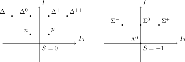which looks similar to the possible states of spin-0, spin-1/2, spin-1, and spin-3/2 particle.

Three flavors (or generations) of fermions form flavor symmetry of SU(3), which is then broken by the unequal Yukawa coupling.

In Schrödinger picture the state evolves while the operator is fixed: \[ \hat{x}, \hat{p}, \quad \ket{\psi(\mathbf{x})}(t) = e^{-i\hat{H}t/\hbar}\ket{\psi(\mathbf{x})}. \]

While in Heisenberg picture the operator evolves and the state remain fixed: \[ \hat{x}(t) = e^{i\hat{H}t/\hbar}\hat{x}e^{-i\hat{H}t/\hbar}, \hat{p}(t) =e^{i\hat{H}t/\hbar}\hat{p}e^{-i\hat{H}t/\hbar}, \quad\ket{\psi(\mathbf{x})}. \] The operator "predict" the future state from the current state.

It is easy to see why Heisenberg picture is preferred in quantum field theory, when you try to express the state of a quantum field: \[ \hat{\phi}(\mathbf{x}), \quad \ket{\psi(\phi)}(t) = e^{-i\hat{H}t/\hbar}\ket{\psi(\phi)}. \] Every field variable operator at each point \( \mathbf{x} \) is fixed in time, and the wave function defined over the space of every possible field evolves. It is clear that we cannot evolve this beast directly, so we choose get around this with \[ \hat{\phi}(\mathbf{x}, t) = e^{i\hat{H}t/\hbar}\hat{\phi}(\mathbf{x})e^{-i\hat{H}t/\hbar}, \quad \ket{\psi(\phi)}. \]

• Field operator: \( \phi(x) \).
• Canonical momentum operator: \( \Pi(x) \).
• Creation and annihilation operators: \( a^{\dagger}(\mathbf{x}), a(\mathbf{x}). \)
  • They are defined by the \( \phi(\mathbf{x}, 0), \Pi(\mathbf{x}, 0) \), so they are constant operators by definition.
• The Lagrangian density operator \( \mathcal{L} \) and Hamiltonian density operator: \( \mathcal{H} \).

Operators that acts only on a single mode, which can be obtained by the Fourier transform of the operators per position.

The creation operator excite the vacuum state with a plane wave that represent a single particle: \[ \ket{\mathbf{k}} := a^{\dagger}(\mathbf{k})\ket{0}. \] They are normalized to satisfy \[ \braket{\mathbf{k}}{\mathbf{k}'} = (2\pi)^3 \delta^{(3)}(\mathbf{k} - \mathbf{k}'). \]

However, these are not Lorentz covariant, so we add additional factor: \[ \ket{k} := \sqrt{2\omega_{\mathbf{k}}} \ket{\mathbf{k}}. \] Now with the normalization given by \[ \braket{k}{k'} = 2\omega_{\mathbf{k}} (2\pi)^3\delta^{(3)}(\mathbf{k} - \mathbf{k}'), \] and the state transforms nicely: \[ U_{\Lambda}\ket{k} = \ket{\Lambda k}. \] (p set 3)

In general, a single-particle state is given by: \[ \ket{\psi} = \int \frac{\dd[3]{\mathbf{k}}}{(2\pi)^3} f(\mathbf{k}) \ket{k}, \] and many-particle state like: \[ \ket{\phi} = \int \frac{\dd[3]{\mathbf{k}_1}}{(2\pi)^3}\frac{\dd[3]{\mathbf{k}_2}}{(2\pi)^3} \cdots \frac{\dd[3]{\mathbf{k}_n}}{(2\pi)^3} f(\mathbf{k}_1, \mathbf{k}_2, \dots, \mathbf{k}_n) \ket{k_1, k_2, \dots, k_n}. \]

S-matrix is an infinite matrix that give information about which interaction is happening at which rate. The \( S_{\alpha\beta} \) entry is given by: \[ S_{\alpha\beta} = \lim_{\begin{smallmatrix}t \to \infty \\ t' \to -\infty \end{smallmatrix}}\mel{\beta}{e^{-i\hat{H}(t - t')/\hbar}}{\alpha}. \] This is the transition amplitude from state \( \alpha \) at \( t = -\infty \) to state \( \beta \) at \( t = \infty \), with the assumption that

• \( \alpha \) and \( \beta \) are localized states in which each particle can be discerned,
• the localized wave packets are infinitely far apart.

Each state is given as a set of momentums. When there is no interaction S-matrix would be an identity. Assuming small interaction, we can write: \[ S_{\alpha\beta} = \delta_{\alpha\beta} + iT_{\alpha\beta}. \] From energy-momentum conservation, we can express \( T_{\alpha\beta} \) as: \[ T_{\alpha\beta} = (2\pi)^4 \delta^{(4)}(p_{\alpha} - p_{\beta}) M_{\alpha\to \beta} \] where \( p_{\alpha}, p_{\beta} \) are the total four-momentum of each state, and \( M_{\alpha\to\beta} \) is called the scattering amplitude.

The scattering amplitude \( M_{\alpha\to\beta} \) can be obtained from time-ordered correlation function: \[ M_{\alpha\to\beta} = \ev{\mathrm{T}\phi(x_1) \cdots \phi(x_n)}{\Omega} \] where \( \mathrm{T} \) is the time-ordering that means the operator next to them has to be reordered with respect to time, and \( \ket{\Omega} \) is the vacuum state of non-free Lagrangian.

• Scalar Free Field

The Klein-Gordon Lagrangian for a complex scalar (spin-0) field \( \phi \) is \[ \mathcal{L} = \partial^{\mu}\phi \partial_{\mu}\phi^* - m^2\phi^* \phi \] in mostly positive metric.

This is the simplest Lagrangian that is

• local: only in terms of local quantities such as \( \phi, \partial_{\mu}\phi \),
• first order derivative in time (from experience),
• Lorentz invariant.

Using the natural units, the classical equation of motion can be written as: \[ (\partial^{\mu}\partial_{\mu} + m^2)\phi = 0. \]

The solution can be easily found using the correpondence between the algebra of classical quantities and the algebra of observables within linear order: \[ \phi(x) = \int \frac{\dd[3]{\mathbf{k}}}{(2\pi)^3} \frac{1}{\sqrt{2\omega_{\mathbf{k}}}} \left(a(\mathbf{k}) e^{-i\omega_{\mathbf{k}}t + i\mathbf{k}\vdot \mathbf{x}} + a^{\dagger}(\mathbf{k}) e^{i\omega_{\mathbf{k}}t - i\mathbf{k}\vdot \mathbf{x}}\above right). \] This operator will detect and evolve each \( \mathbf{k} \) eigenstate of the initial state, and find the field variable at \( x \).

• Spinor Free Field

\[ \tau = \frac{1}{\Gamma}. \]

It is a probabilistic process of tunneling out of the potential well of the strong force.

The element above right the iron is technically unstable, but the energy of the alpha particle within the neucleus is so small that the probalitity of tunneling is minute compared to the highly unstable ones.

\begin{align*} \mathcal{L}_{\rm fermion} + \mathcal{L}_{\rm gauge} = \sum_{j = 1,2,3} &\left( \bar{q}_{\mathrm{L}j}i \gamma^{\mu} D_{\mu} q_{\mathrm{L}j} + \bar{u}_{\mathrm{R}j}i\gamma^{\mu}D_{\mu}u_{\mathrm{R}j} + \bar{d}_{\mathrm{R}j} i \gamma^{\mu}D_{\mu} d_{\mathrm{R}j} + \bar{\ell}_{\mathrm{L}j} i\gamma^{\mu} D_{\mu} \ell_{\mathrm{L}j} + \bar{e}_{\mathrm{R}j} i\gamma^{\mu} D_{\mu}e_{\mathrm{R}j} \above right) \\ - \frac{1}{4} &B_{\mu\nu}B^{\mu\nu} - \sum_{a=1,2,3} \frac{1}{4} W^a_{\mu\nu}W^{a\mu\nu} - \sum_{A=1,\dots, 8} \frac{1}{4} G^A_{\mu\nu}G^{A\mu\nu} \end{align*}

where \(j\) enumerates the flavors (or generations), \(A\) enumerates the generators of SU(3), \(a\) enumerators the generators of SU(2), \[ q_\mathrm{L} = \begin{pmatrix} u_\mathrm{L} \\ d_\mathrm{L} \end{pmatrix} \] is doublet of left-handed Weyl spinors of up quark \(u_\mathrm{L}\) and down quark \(d_\mathrm{L}\) (up to flavor), \[ \ell_\mathrm{L} = \begin{pmatrix} \nu_\mathrm{L} \\ e_\mathrm{L} \end{pmatrix} \] is doublet of left-handed Weyl spinors of neutrino \(\nu_\mathrm{L}\) and electron \(e_\mathrm{L}\) (up to flavor), \(u_\mathrm{R}, d_\mathrm{R}, \nu_\mathrm{R}, e_\mathrm{R}\) are the singlets of above right-handed Weyl spinor for respective particles, \(\gamma^{\mu}\) is gamma matrices, \(D_{\mu}\) is the covariant derivative operator given by described separately, \(B_{\mu\nu}\) is the field strength tensor of photon (before electroweak symmetry breaking) field given by: \[ B_{\mu\nu} = \partial_{\mu}B_{\nu} - \partial_{\nu}B_{\mu}, \] \(W_{\mu\nu}^a\) are the field strength tensors of W boson (before electroweak symmetry breaking) fields \(W_{\mu}^a\) given by: \[ W^a_{\mu\nu} = \partial_{\mu}W^a_{\nu} - \partial_{\nu}W^a_{\mu} + g \epsilon^{abc}W^{b}_{\mu}W^{c}_{\nu}, \] \(G^A_{\mu\nu}\) are the field strength tensors of gluon fields \(G_{\mu}^A\) given by: \[ G^A_{\mu\nu} = \partial_{\mu}G^A_{\nu} - \partial_{\nu}G^A_{\mu} + g_s f^{ABC}G^B_{\mu}G^C_{\nu}. \]

\begin{align*} \mathcal{L}_{\rm Higgs} &= (D^{\mu}h)^{\dagger}D_{\mu}h - \lambda \left( h^{\dagger}h - \frac{v^2}{2} \above right)^2 \\ \mathcal{L}_{\rm Yukawa} &= - y_{\rm u}^{ij}\epsilon^a{}_bh^{\dagger b} \bar{q}_{\mathrm{L} ia}u_{\mathrm{R}j}^\mathsf{c} - y_{\rm d}^{ij} h^a \bar{q}_{\mathrm{L} ia} d_{\mathrm{R} j}^{\mathsf{c}} - y_{\rm e}^{ij} h^a \bar{\ell}_{\mathrm{L} ia} e_{\mathrm{R} j}^{\mathsf{c}} + \text{h.$\,$c.} \end{align*}

where \(i,j\) enumerates the flavors, \(a,b\) enumerates the components of SU(2), \[ h = \begin{pmatrix} h_1 \\ h_2 end{pmatrix} \] is doublet of complex scalar fields, \(\lambda\) is a scalar parameter, \(v\) is the vacuum expectation value of Higgs field, \(y_{\mathrm{u}}, y_{\mathrm{d}}, y_{\mathrm{e}}\) are the Yukawa coupling matrices that couples different generations, \(\psi^{\mathsf{c}} := C \bar{\psi}^{\mathsf{T}}\) is the charge conjugate of Weyl spinor.

\begin{align*} \mathcal{L}_{\mathrm{SM}} ={}& -\frac{1}{2}\partial^\nu g^{a\mu}\partial_\nu g_{a\mu} -g_s f^{abc}\partial^\mu g^{a\nu}g_\mu^b g_\nu^c -\frac{1}{4}g_s^2 f^{abc}f^{ade}g^{b\mu}g^{c\nu}g_\mu^d g_\nu^e \\[1ex] &-\partial^\nu W^{+\mu}\partial_\nu W_\mu^- +m_W^2 W^{+\mu}W_\mu^- -\frac{1}{2}\partial^\nu Z^{0\mu}\partial_\nu Z_\mu^0 +\frac{m_W^2}{2c_w^2}Z^{0\mu}Z_\mu^0 -\frac{1}{2}\partial^\nu A^\mu\partial_\nu A_\mu +\frac{1}{2}\partial^\mu H\partial_\mu H -\frac{1}{2}m_H^2 H^2 \\ &+\partial^\nu\phi^+\partial_\nu\phi^- -m_W^2\phi^+\phi^- +\frac{1}{2}\partial^\nu\phi^0\partial_\nu\phi^0 -\frac{m_W^2}{2c_w^2}(\phi^0)^2 -\beta_H\left[ \frac{2m_W^2}{g^2}+\frac{2m_W}{g}H +\frac{1}{2}\left(H^2+(\phi^0)^2+2\phi^+\phi^-\above right) \above right] +\frac{2m_W^4}{g^2}\alpha_H \\ &-igc_w\left[ \partial^\nu Z^{0\mu}\left(W_\mu^+W_\nu^- - W_\nu^+W_\mu^-\above right) -Z^{0\nu}\left(W^{+\mu}\partial_\nu W_\mu^- - W^{-\mu}\partial_\nu W_\mu^+\above right) +Z^{0\mu}\left(W^{+\nu}\partial_\nu W_\mu^- - W^{-\nu}\partial_\nu W_\mu^+\above right) \above right] \\ &-igs_w\left[ \partial^\nu A^\mu\left(W_\mu^+W_\nu^- - W_\nu^+W_\mu^-\above right) -A^\nu\left(W^{+\mu}\partial_\nu W_\mu^- - W^{-\mu}\partial_\nu W_\mu^+\above right) +A^\mu\left(W^{+\nu}\partial_\nu W_\mu^- - W^{-\nu}\partial_\nu W_\mu^+\above right) \above right] \\ &-\frac{1}{2}g^2 W^{+\mu}W_\mu^-W^{+\nu}W_\nu^- +\frac{1}{2}g^2 W^{+\mu}W^{-\nu}W_\mu^+W_\nu^- +g^2c_w^2\left( Z^{0\mu}W_\mu^+Z^{0\nu}W_\nu^- -Z^{0\mu}Z_\mu^0W^{+\nu}W_\nu^- \above right) \\ &+g^2s_w^2\left( A^\mu W_\mu^+A^\nu W_\nu^- -A^\mu A_\mu W^{+\nu}W_\nu^- \above right) +g^2s_wc_w\left[ A^\mu Z^{0\nu}\left(W_\mu^+W_\nu^-+W_\nu^+W_\mu^-\above right) -2A^\mu Z_\mu^0W^{+\nu}W_\nu^- \above right] \\ &-g\alpha_Hm_W\left[ H^3+H(\phi^0)^2+2H\phi^+\phi^- \above right] -\frac{1}{8}g^2\alpha_H\left[ H^4+(\phi^0)^4+4(\phi^+\phi^-)^2 +4(\phi^0)^2\phi^+\phi^- +2H^2(\phi^0)^2+4H^2\phi^+\phi^- \above right] \\ &+gm_WW^{+\mu}W_\mu^-H +\frac{1}{2}g\frac{m_W}{c_w^2}Z^{0\mu}Z_\mu^0H +\frac{1}{2}ig\left[ W^{+\mu}\left(\phi^0\partial_\mu\phi^- - \phi^-\partial_\mu\phi^0\above right) -W^{-\mu}\left(\phi^0\partial_\mu\phi^+ - \phi^+\partial_\mu\phi^0\above right) \above right] \\ &-\frac{1}{2}g\left[ W^{+\mu}\left(H\partial_\mu\phi^- - \phi^-\partial_\mu H\above right) +W^{-\mu}\left(H\partial_\mu\phi^+ - \phi^+\partial_\mu H\above right) \above right] -\frac{1}{2}\frac{g}{c_w}Z^{0\mu} \left(H\partial_\mu\phi^0-\phi^0\partial_\mu H\above right) \\ &+ig\frac{s_w^2}{c_w}m_WZ^{0\mu} \left(W_\mu^+\phi^- - W_\mu^-\phi^+\above right) -igs_wm_WA^\mu \left(W_\mu^+\phi^- - W_\mu^-\phi^+\above right) \\ &+ig\frac{s_w^2-c_w^2}{2c_w}Z^{0\mu} \left(\phi^+\partial_\mu\phi^- - \phi^-\partial_\mu\phi^+\above right) -igs_wA^\mu \left(\phi^+\partial_\mu\phi^- - \phi^-\partial_\mu\phi^+\above right) \\[1ex] &+\frac{1}{4}g^2W^{+\mu}W_\mu^- \left[H^2+(\phi^0)^2+2\phi^+\phi^-\above right] +\frac{1}{8}\frac{g^2}{c_w^2}Z^{0\mu}Z_\mu^0 \left[H^2+(\phi^0)^2+2(s_w^2-c_w^2)\phi^+\phi^-\above right] \\ &+\frac{1}{2}g^2\frac{s_w^2}{c_w}Z^{0\mu}\phi^0 \left[W_\mu^+\phi^-+W_\mu^-\phi^+\above right] +\frac{1}{2}ig^2\frac{s_w^2}{c_w}Z^{0\mu}H \left[W_\mu^+\phi^- - W_\mu^-\phi^+\above right] -\frac{1}{2}g^2s_wA^\mu\phi^0 \left[W_\mu^+\phi^-+W_\mu^-\phi^+\above right] \\ &-\frac{1}{2}ig^2s_wA^\mu H \left[W_\mu^+\phi^- - W_\mu^-\phi^+\above right] +g^2\frac{s_w}{c_w}(c_w^2-s_w^2)A^\mu Z_\mu^0\phi^+\phi^- +g^2s_w^2A^\mu A_\mu\phi^+\phi^- \\[1ex] &+\bar e^\sigma\left(i\gamma^\mu\partial_\mu-m_e^\sigma\above right)e^\sigma +\bar\nu^\sigma i\gamma^\mu\partial_\mu\nu^\sigma +\bar d_j^\sigma\left(i\gamma^\mu\partial_\mu-m_d^\sigma\above right)d_j^\sigma +\bar u_j^\sigma\left(i\gamma^\mu\partial_\mu-m_u^\sigma\above right)u_j^\sigma \\ &+gs_wA^\mu\left[ -\left(\bar e^\sigma\gamma_\mu e^\sigma\above right) -\frac{1}{3}\left(\bar d_j^\sigma\gamma_\mu d_j^\sigma\above right) +\frac{2}{3}\left(\bar u_j^\sigma\gamma_\mu u_j^\sigma\above right) \above right] +\frac{g}{4c_w}Z^{0\mu}\Biggl[ \left(\bar\nu^\sigma\gamma_\mu(1-\gamma^5)\nu^\sigma\above right) +\left(\bar e^\sigma\gamma_\mu\left(4s_w^2-(1-\gamma^5)\above right)e^\sigma\above right) \\ &\qquad +\left(\bar d_j^\sigma\gamma_\mu \left(\frac{4}{3}s_w^2-(1-\gamma^5)\above right)d_j^\sigma\above right) +\left(\bar u_j^\sigma\gamma_\mu \left(-\frac{8}{3}s_w^2+(1-\gamma^5)\above right)u_j^\sigma\above right) \Biggr] \\ &+\frac{g}{2\sqrt{2}}W^{+\mu}\left[ \left(\bar\nu^\sigma\gamma_\mu(1-\gamma^5)P^{\sigma\tau}e^\tau\above right) +\left(\bar u_j^\sigma\gamma_\mu(1-\gamma^5)C^{\sigma\tau}d_j^\tau\above right) \above right] \\ &+\frac{g}{2\sqrt{2}}W^{-\mu}\left[ \left(\bar e^\sigma\gamma_\mu(1-\gamma^5)P^{\dagger\,\sigma\tau}\nu^\tau\above right) +\left(\bar d_j^\sigma\gamma_\mu(1-\gamma^5)C^{\dagger\,\sigma\tau}u_j^\tau\above right) \above right] \\[1ex] &+i\frac{g}{2\sqrt{2}}\frac{m_e^\sigma}{m_W}\left[ -\phi^+\left(\bar\nu^\sigma(1+\gamma^5)e^\sigma\above right) +\phi^-\left(\bar e^\sigma(1-\gamma^5)\nu^\sigma\above right) \above right] -\frac{g}{2}\frac{m_e^\sigma}{m_W} \left[H\bar e^\sigma e^\sigma-i\phi^0\bar e^\sigma\gamma^5e^\sigma\above right] \\ &+i\frac{g}{2\sqrt{2}m_W}\phi^+\left[ -m_d^\tau\left(\bar u_j^\sigma C^{\sigma\tau}(1+\gamma^5)d_j^\tau\above right) +m_u^\tau\left(\bar u_j^\sigma C^{\sigma\tau}(1-\gamma^5)d_j^\tau\above right) \above right] \\ &+i\frac{g}{2\sqrt{2}m_W}\phi^-\left[ m_d^\tau\left(\bar d_j^\sigma C^{\dagger\,\sigma\tau}(1-\gamma^5)u_j^\tau\above right) -m_u^\tau\left(\bar d_j^\sigma C^{\dagger\,\sigma\tau}(1+\gamma^5)u_j^\tau\above right) \above right] \\ &-\frac{g}{2}\frac{m_u^\sigma}{m_W}H\bar u_j^\sigma u_j^\sigma -\frac{g}{2}\frac{m_d^\sigma}{m_W}H\bar d_j^\sigma d_j^\sigma -i\frac{g}{2}\frac{m_u^\sigma}{m_W}\phi^0\bar u_j^\sigma\gamma^5u_j^\sigma +i\frac{g}{2}\frac{m_d^\sigma}{m_W}\phi^0\bar d_j^\sigma\gamma^5d_j^\sigma \\[1ex] &-\frac{1}{2}ig_s\bar d_i^\sigma\gamma^\mu\lambda_{ij}^a d_j^\sigma g_\mu^a -\frac{1}{2}ig_s\bar u_i^\sigma\gamma^\mu\lambda_{ij}^a u_j^\sigma g_\mu^a \\[1ex] &-\bar X^+\left(\partial^\mu\partial_\mu+m_W^2\above right)X^+ -\bar X^-\left(\partial^\mu\partial_\mu+m_W^2\above right)X^- -\bar X^0\left(\partial^\mu\partial_\mu+\frac{m_W^2}{c_w^2}\above right)X^- -\bar Y\partial^\mu\partial_\mu Y \\ &-igc_wW^{+\mu} \left(\partial_\mu\bar X^0X^- - \partial_\mu\bar X^+X^0\above right) -igs_wW^{+\mu} \left(\partial_\mu\bar YX^- - \partial_\mu\bar X^+Y\above right) \\ &-igc_wW^{-\mu} \left(\partial_\mu\bar X^-X^0-\partial_\mu\bar X^0X^+\above right) -igs_wW^{-\mu} \left(\partial_\mu\bar X^-Y-\partial_\mu\bar YX^+\above right) \\ &-igc_wZ^{0\mu} \left(\partial_\mu\bar X^+X^+-\partial_\mu\bar X^-X^-\above right) -igs_wA^\mu \left(\partial_\mu\bar X^+X^+-\partial_\mu\bar X^-X^-\above right) \\ &-\frac{1}{2}gm_W\left[ \bar X^+X^+H+\bar X^-X^-H+\frac{1}{c_w^2}\bar X^0X^0H \above right] \\ &+\frac{s_w^2-c_w^2}{2c_w}igm_W \left[\bar X^+X^0\phi^+-\bar X^-X^0\phi^-\above right] +\frac{1}{2c_w}igm_W \left[\bar X^0X^-\phi^+-\bar X^0X^+\phi^-\above right] \\ &+igm_Ws_w\left[\bar X^-Y\phi^- - \bar X^+Y\phi^+\above right] +i\frac{1}{2}gm_W\left[\bar X^+X^+\phi^0-\bar X^-X^-\phi^0\above right] \\[1ex] &-\bar G^a\partial^\mu\partial_\mu G^a -g_sf^{abc}\partial^\mu\bar G^aG^b g_\mu^c \end{align*}